Spm Add Maths Formula List Form5 603sl
This document was ed by and they confirmed that they have the permission to share it. If you are author or own the copyright of this book, please report to us by using this report form. Report 2z6p3t
Overview 5o1f4z
& View Spm Add Maths Formula List Form5 as PDF for free.
More details 6z3438
- Words: 3,768
- Pages: 28
Additional Mathematics
Formulae List Form 5 (prepared by:BEHPC)
1
01 Progressions Arithmetic Progression
Geometric Progression
1. Common Difference
1. Common Ratio
d =Tn −Tn −1
r=
2. The nth term
Tn Tn −1
2. The nth term Tn =a +(n −1)d
Tn = ar n −1
3. Sum of the first n Sn =
3. Sum of the first n
n [ 2a + (n −1)d ] 2
Sn =
or Sn =
n [ a +l] 2
Sn =
where l = last term
(
) , r ≠1
a r n −1 r −1
(
a 1−rn 1− r
for r > 1
) , r ≠ 1, for r < 1
4. Sum to infinity: S∞ =
If Sn is given as a function of n, then use: Tn = Sn −S n−1
First term, Second term,
a = T1 = S1
T2 = S 2 − S1
Sum of the from mth term to nth term:) Sum = S n − S m−1
(For example –The sum from 3rd term to 7th term, Sum = S7 − S2 )
2
a , 1− r
r <1
02 Linear Law 1.
Drawing lines of best fit Line of best fit has 2 characteristics: it es through as many points as possible, the number of points which are not on the line of best fit are equally distributed on the both sides of the line.
Recall: (1) Equation of a straight line if two points are given:
(2) Equation of a straight line if m and c are given: Steps to draw a line of best fit: Construct a table consisting the given variables. Plot a graph of Y against X , using the scale specified AND draw a line of best fit. Calculate the gradient, m, and get the Yintercept, c, from the graph. Re-write the original equation given and reduce it to linear form. Compare with values of m and c obtained, find the values of the unknowns required.
2.
3.
To reduce nonlinear functions to linear form
Tips: (1)
The equation must have one constant (without x and y). (2) Y cannot have constant, but can have x and y. (3) X cannot have y., but can have x and constant.
Equations of lines of best fit A set of two variables are related non linearly can be converted to a linear equation. The line of best fit can be written in the form
where X and Y are in of x and/or y m is the gradient, c is the Y-intercept The graph of can be used to find the values of constants of the non-linear equation and others information relating the two variables.
3
The table shows some of examples of non-linear equations can be reduced to the linear form: Non-linear equation 2
y = px + qx
q y = px + x q y= p x+ x p q = +1 y x x y= p + qx
Linear equation y = px + q x y q = +p x2 x xy = px 2 + q y q = +p x x2 y x = px + q y q = +p x x 1 q 1 = + y px p 1 1 = p ÷+ q y x
Y y x y x2 xy y x y x y x 1 y 1 y
X
m
c
x
p
q
1 x
q
p
p
q
q
p
p
q
q
p
q p
1 p
p
q
x
3 p
3q p
x2 1 x2 x 1 x 1 x 1 x
y = pq x
3 3q y = ÷x + p p log10 y = x log10 q + log10 p
log10 y
x
log10 q
log10 p
y = px q
log10 y = q log10 x + log10 p
log10 y
log10 x
q
log10 p
y = pq x +1
log10 y = ( x + 1)log10 q + log10 p
log10 y
x +1
log10 q
log10 p
y=
9 ( x + q)2 p2
4
y
03 Integration Integration is the inverse process of differentiation. If , then where c = constant. Indefinite integrals:(Refer to the examples below after note 6) (a) (b) (c) 3.
Definite integrals
The laws of definite integrals:
(a) (b) (c) (d) (e)
4.
Finding Equation Of A Curve From Its Gradient Function: Differentiati on Gradient function
The equation of the curve
Integration
y = ∫ f ' ( x) dx
5
5.
Integration As The Summation Of Areas: Area bounded by the curve y= f(x),the lines x = a, x = b and the x-axis
Area bounded by the curve x = f(y), the lines y = a, y = b and the y-axis.
b
A = ∫ xdy
b
a
A = ∫ ydx a
Area of the region between a curve y = f(x) and a straight line y = g(x)
A=
b
b
a
a
∫ f ( x)dx − ∫ g ( x)dx
6
6.
Integration As The Summation Of Volumes
The volume of the solid generated when the region enclosed by the curve y = f(x), the x-axis, the line x = a and the line x = b is revolved through 360° about the x-axis is given by
b
The volume of the solid generated when the region enclosed by the curve x = f(y), the y-axis, the line y = a and the line y = b is revolved through 360 ° about the y-axis is given by
b
V y = ∫ π x 2 dy
V x = ∫ π y dx 2
a
a
Refer to Note 3: Example: Example:
∫ (u ± v)dx = ∫ udx ±∫ vdx
Example: 1 x −4 −5 dx = x dx = +c ∫ x5 ∫ −4
u and v are functions in x
Example: 2 2 ∫ 3x + 2 xdx = ∫ 3x dx + ∫ 2 xdx 1.
Example:
=
3x3 2 x 2 3 x3 2 x 2 + +c = + +c 3 2 3 2
= x3 + x 2 + c
7
Example: 2 2 −5 2 x −4 dx = x dx = ( )+c ∫ 3x5 ∫3 3 −4 2 x −4 x −4 = ( )+c = +c 3 −4 −6
Example:
Example:
Example:
8
04 Vectors
9
Vector is a quantity that has both magnitude and direction. Scalar is a quantity that has magnitude only. A vector can be presented by a line segment with an arrow, known as a directed line segment.
Negative vector of has the same magnitude as but its direction is opposite to .
A zero vector ia a vector whose magnitude is zero. It is denoted by . Two vectors are equal if both the vectors have the same magnitude and direction. When a vector is multiplied by a scalar , the product is . Its magnitude is times the magnitude of the vector . The vector is parallel to the vector if and only if , where is a constant. If the vectors and are not parallel and , then and . Addition of vectors Triangle Law
Parallelogram Law
The subtraction of the vector from the vector is written as . This operation can be considered as the addition of the vector with the negative vector of , i.e. .
10
Column vector:
A unit vector is a vector whose magnitude is one unit. The magnitude of the vector can be calculated using the Pythagoras’ Theorem.
(i) To show is parallel to , To show A, B and C are collinear, To find the ratio of AB :BC
uuurUseuuur AB = k BC
11
05 Trigonometric Functions Positive and Negative Angles Positive angles are angles measure in an anticlockwise rotate from the positive x-axis about the origin, O.
Complementary Angle sin θ = cos(90° − θ ) cosθ = sin(90° − θ ) tan θ = cot(90° − θ ) cot θ = tan(90° − θ ) secθ = cosec(90° − θ ) cosecθ = sec(90° − θ )
Negative angles are angles measured in a clockwise rotation from the positive x-axis about the origin O.
Negative Angle sin(−θ ) = − sin θ cos(−θ ) = cos θ tan(−θ ) = − tan θ
Six Trigonometric Functions of Any Angle
sin θ =
y r
tan θ =
cosθ = sin θ cosθ
sec θ =
1 cosθ
x r
cot θ =
tan θ =
Positive/Negative sign at different quadrant
y x
A
T
C
Just the positive ratio!!! cos x
sin x
1 cos θ = tan θ sin θ
cosecθ =
S
1 sin θ
tan x
12
1
cot x
sec x
cot x
13
Value of Special Angle 30o and 60o
sin 30° =
1 2
sin 60° =
3 2
cos30° = 3 2
cos 60° =
1 2
tan 30° =
θ cos θ
0o 1
90o 0
180o -1
270o 0
360o 1
θ tan θ
0o 0
90o ∞
180o 0
270o ∞
360o 0
Alternative Way: 0o 30o θ
45o
60o
90o
2 2 2 2 2 2 2 2
3 2 3 2 1 2 1 2
4 2
1
3
1 3
tan 60° = 3
Value of Special Angle 45o
sin θ
1 sin 45° = 2
1 cos 45° = 2
0 2
0 tan 45°=1
cosθ
4 2
1 Value of Special Angle 0o, 90o, 180o, 270o, 360o.
θ sin θ
0o 0
90o 1
180o 0
270o -1
tan θ
0
1 2 1 2 3 2 3 2 1 3
1 0 2
0 ∞
Steps to solve simple trigonometric equation: (1) Determine the range of values of the required angles. (2) Find a basic angle by using calculator. (3) Determine the quadrants the angle should be. (4) Determine the values of angles in those quadrants.
360o 0
14
Graphs of The Functions of Sine, Cosine and Tangent Graph of.y = sin x
x sin
0o 0
90o 1
180o 0
270o -1
360o 0
180o -1
270o 0
360o 1
270o ∞
360o 0
Graph of.y = cos x
x cos x
0o 1
90o 0
Graph of.y = tan x
x tan x
15
0o 0
90o ∞
180o 0
cos 2 A =2 cos 2 A −1
or
cos 2 A =1 −2 sin 2 A
Basic Trigonometric Identities:
tan 2 A =
sin 2 x +cos 2 x =1
2 tan A 1 − tan 2 A
tan 2 x +1 =sec 2 x cot 2 x +1 =cosec 2 x
Half Angle Formulae: sin A = 2sin
A A cos 2 2
cos A = cos 2
A A − sin 2 2 2
cos A = 2 cos 2
A −1 2
cos A = 1 − 2 sin 2
Compound AnglesFormulae:
For right angled triangle, use:
sin( A ±B) =sin A cos B ±cos A sin B cos( A ±B ) =cos A cos B msin A sin B
tan( A ± B) =
tan A ± tan B 1 mtan A tan B
Double Angle Formulae: sin 2 A =2 sin A cos A
cos 2 A =cos 2 A −sin 2 A
A 2
or
A 2 tan A = 2 A 1 − tan 2 2 tan
16
or
or
06 Permutations and Combinations The number of permutations of n different objects, taken r at a time is given by :
Multiplication Principle / Rule If an operation can be carried out in r ways and another operation can be carried out in s ways, then the number of ways to carry out both the operations consecutively is r ×s, i.e. rs. The rs multiplication principle can be expanded to three or more operations. If the numbers of ways for the occurrence of events A, B and C are r, s and p respectively, the number of ways for the occurrence of all the three events consecutively is r × s × p, i.e. rsp.
A permutation of n different objects, taken r at a time, is an arrangement of a set of r objects chosen from n objects. The order of the objects in the chosen set is taken into consideration. The number of permutations of n different objects, taken all at a time, is : Note: (i) (ii) (iii)
Permutations The number of permutations of n different objects is n!, where
n!, is read as n factorial.
Combinations
Permutation of n Different Objects, Taken r at a Time
17
The number of combinations of r objects chosen from n different objects is given by :
A combination of r bjects chosen from n different objects is a selection of a set of r objects chosen from n objects. The order of the objects in the chosen set is not taken into consideration. Note: (i) (ii) (iii) (iv)
18
07 Probability 1. The probability for the occurrence of an event A in the sample space S is P ( A) =
number of outcomes of event A number of outcomes of sample space S
P( A) =
n( A) n( S )
2. (a) The range of values of a probability is 0 ≤ P ( A) ≤ 1 . (b) If P(A) = 1, event A is sure to occur. (c) If P(A) = 0, event A will not occur. 3. The complement of an event A is denoted by A and the probability of a complementary event is given by
P ( A) = 1 − P ( A) 4. The probability for the occurrence of events A or B or both is P( A ∪ B ) = P ( A) +P ( B ) −P ( A ∩B )
5.
If the events A and B are mutually exclusive, then A ∩ B = ∅ and P( A ∩ B ) = 0 . Thus, P( A ∪ B ) = P ( A) +P ( B )
6. The probability of the combination of two independent events, A and B, if the occurrence or nonoccurrence of one event does not affect of the other is given by P( A ∩ B ) =P ( A) ×P ( B )
7. The concept of the probability of two independent events can be expanded to three or more independent events. If A, B and C are three independent events, the probability for the occurrence of events A, B and C is P ( A ∩B ∩ C ) =P ( A) ×P ( B ) ×P (C )
8. A tree diagram can be constructed to show all the possible outcomes of an experiment.
19
08 Probability Distributions PROBABILITY DISTRIBUTIONS
NORMAL DISTRIBUTIONS
BINOMIAL DISTRIBUTIONS 1. A random variable that has finite and countable values is known as a discrete random variable. 2. For a Binomial Distribution, the probability of obtaining r numbers of successes out of n experiments is given by where P = probability X = discrete random variable r = number of success (0, 1, 2, 3, …,n) n = number of trials p = probability of success in an experiment (0 < p <1) q = probability of failure in an experiment ( ) 3. A binomial probability distribution can be plotted as a graph. 4. Determine the mean, variance and standard deviation of binomial distribution If X is a binomial discrete random variable such that X~B (n, p), then Mean of X, Variance of X, Standard deviation of X,
20
Continuous random variable is a variable that can take any infinite value in a certain range. A normal distribution is a probability distribution of continuous random variables (only quantities that can be measured).The distribution is denoted by where = mean and = variance. A normal distribution with =0 and = 1 is known as a standard normal distribution and is denoted by N (0,1). A normal random variable, X, can be converted into standard normal random variable by using . Z= X=
µ= σ =
standard score or z-score value of a normal random variable mean of a normal distribution standard deviation of a normal distribution
Normal Distribution 1. A continuous random variable, X, is normally distributed if the graph of its probability function has the following properties.
• • •
Its curve has a bell shape and it is symmetrical at the line x = µ. Its curve has a maximum value at x = µ. The area enclosed by the normal curve and the x-axis is 1.
09 Motion Along a Straight Line 9.1
Displacement
1. (a) Positive displacement means that the particle is at the right-hand side of O. (b) Negative displacement means that the particle is at the left-hand side of O. (c) Zero displacement means that the particle is at O. 2. Total distance travelled in the first n seconds is the total distance travelled by a particle from time t = 0 to t = n. 3. Distance travelled during the nth second is the distance travelled by the particle from time t = (n – 1) to t = n. Thus, Distance travelled during the nth second = Sn − Sn−1
9.2
Velocity
1. Instantaneous velocity, v, is the rate of change of displacement, s, with respect to time, t and it is given by
v=
ds dt
2. (a) When a particle moves to the right, it has a positive velocity. (b) When a particle moves to the left, it has a negative velocity. (c) When a particle is instantaneously at rest, it has a zero velocity. 3. The displacement of particle is a maximum (to the right or to the left of the fixed point O) when its velocity is zero.
21
4. A particle reverses its direction when it comes to instantaneous rest, i.e. v = 0. 5. Displacement, s, is given by the integration of the instantaneous velocity, v, with respect to time, t, i.e.
n
6. Distance travelled during the nth second =
∫ v dt
n −1
7. The displacement of particle is a maximum (to the right or to the left of the fixed point O) when its velocity is zero. 8. A particle reverses its direction when it comes to instantaneous rest, i.e. v = 0.
9.3
Acceleration
1. Acceleration is the rate of change of velocity. a=
dv d 2 s = dt dt 2
v = ∫ a dt
2. (a) Positive acceleration means that the velocity is increasing with respect to time. (b) Negative acceleration or deceleration means that the velocity is decreasing with respect to time. (c) Zero acceleration means that the velocity is a constant (uniform velocity). 3. The velocity of a particle is a maximum when its acceleration is zero. 4. The following conclusion can be made.
22
v=
ds dt
s
d 2s a= 2 dt a=
dv dt a
v
v = ∫ a dt
s = ∫ v dt
23
Important tips: Initial displacement / initial velocity / initial acceleration ⇒ (a) at the right-hand side of O ⇒ (b) 4 m to the right of O ⇒ (a) at the left-hand side of O ⇒ (b) 4 m to the left of O ⇒ when the particle moves to the right ⇒ when the particle moves to the left ⇒ when the particle is instantaneously at rest ⇒ when particle reverses its direction ⇒ when the particle returns to O ⇒ maximum displacement of the particle ⇒ or maximum velocity of the particle ⇒ or velocity is increasing / positive acceleration ⇒ velocity is decreasing / negative acceleration ⇒ uniform velocity(velocity is a constant) / zero acceleration ⇒ when particle M and particle N meet ⇒
24
10 Linear Programming 1. Linear programming is a method of solving problems involving two variables that can be represented by a mathematical model by using inequalities as constraints. 2. For ≥ or ≤ , use solid line (). For > or
<,
use dashed line (----).
3. Just how to shade the regions which are greater than: y≥0
(a)
y
y
x
O
(d)
O
x≥a y
y
b
x
O
y ≥ b (b = y-intercept)
(c)
x≥0
(b)
(a = x-intercept)
x= a
y =b x
O
25
a
x
(e)
y ≥ mx + c (m = positive value) (Eg: y ≥ 2 x + 1 ) y y = mx + c
O
y ≥ mx + c (m = negative value) (Eg: y ≥ −2 x + 1 ) y
(f)
y = mx + c
x
O
x
4. A constraint is an inequality that represents a condition that must be satisfied in order for a problem to be solved. Constraint y is more than x y is less than x y is not more than x y is not less than x y is at least k times of x y is at most k times of x The total x and y is not more than 7. k 8. The smallest value of y is k 9. The greatest value of y is k 10. x exceeds two times of y at least k 1. 2. 3. 4. 5. 6.
11. The ratio of y to x is k or more 5. Important keywords:
not less than at least smallest value minimum value
≥
26
Inequality y>x y<x y≤x y≥x y ≥ kx y ≤ kx x+ y ≤k y≥k y≤k x − 2y ≥ k y ≥k x
not more than at most greatest value maximum value
≤
6. Steps to solve a linear programming problem through graphical method: Step 1: Determine the two variables, x and y. Step 2: From the given constraints, interpret the problem and form inequalities that satisfy all the constraints. Step 3: Draw the straight lines for each inequality. Step 4: Determine the region which satisfies all the inequalities. Step 5: Form the optimal function k = ax + by . Step 6: By using a ruler and set square, slide the line towards the region to find the maximum or minimum point based the function. Step 7: Determine the optimal value (maximum or minimum value).
TO MY BELOVED STUDENTS!!!
“GOOD LUCK & ALL THE BEST “ IN YOUR SPM EXAMINATION WISHING YOU THE VERY BEST IN EVERYTHING AND MAY ALL THE NICEST THINGS YOU WISH FOR ALWAYS COME TO YOU. BEST WISHES, PN BEH
27
28
Related Documents c2h70

Spm Add Maths Formula List Form5 603sl
October 2019 28
Spm Add Maths Formula List Form5 603sl
November 2019 38
Spm-add-maths-formula-list-form4 4d3ez
December 2021 0
Spm-add-maths-formula-list-form4.pdf 6o32
December 2019 40
Spm Chemistry Formula List Form5 1x2r24
December 2019 54
Add Maths Sebenar Spm 2005 5e4k1r
November 2021 0More Documents from "Sayantani Ghosh" 22u2z
Spm Add Maths Formula List Form5 603sl
November 2019 38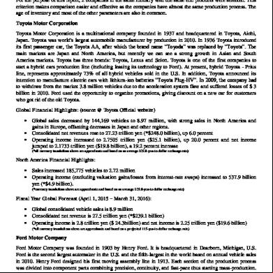
Brief Financial Report On Ford Versus Toyota 6b1z4l
December 2019 25
Power System Analysis By Hadi Saadat Electrical Engineering Libre 5vj4b
April 2020 27
Correction Of Flange Serration 6q5q57
December 2019 27
Analysistabs Project Cost Estimate Template.xls 4c6x5a
November 2019 118